UNIT-3(Gaussian Mixture Model)-MACHINE LEARNING

 

Drawbacks of k-means Clustering

you will notice that all the clusters created are circular. This is because the centroids of the clusters are updated iteratively using the mean value.

Now, consider the following example where the distribution of points is not circular. What do you think will happen if we use k-means clustering on this data? It would still attempt to group the data points circularly. That’s not great! k-means fails to identify the right clusters:

Hence, we need a different way to assign clusters to the data points. So instead of using a distance-based model, we will now use a distribution-based model. And that is where Gaussian Mixture Models come into this article!

Introduction to Gaussian Mixture Models (GMMs)

The Gaussian Mixture Model (GMM) is a probabilistic model used for clustering and density estimation. It assumes that the data is generated from a mixture of several Gaussian components, each representing a distinct cluster. GMM assigns probabilities to data points, allowing them to belong to multiple clusters simultaneously. The model is widely used in machine learning and pattern recognition applications.

Gaussian Mixture Models (GMMs) assume that there are a certain number of components, where each component is a Gaussian distribution. Hence, a Gaussian Mixture Model tends to group the data points belonging to a single Gaussian component together. The parameters of the mixture components, such as the means and covariances, are typically estimated using the Expectation-Maximization (EM) algorithm or maximum likelihood estimation techniques.

Let’s say we have three Gaussian components (more on that in the next section) – GD1, GD2, and GD3. These have a certain mean (μ1, μ2, μ3) and variance (σ1, σ2, σ3) value respectively. For a given set of data points, our GMM would identify the probability of each data point belonging to each of these mixture components. The EM algorithm iteratively updates these parameters to maximize the likelihood of the data, without requiring the derivative to be calculated explicitly.

Wait, probability?

You read that right! Gaussian Mixture Models are probabilistic models and use the soft clustering approach for distributing the points in different clusters. I’ll take another example that will make it easier to understand.

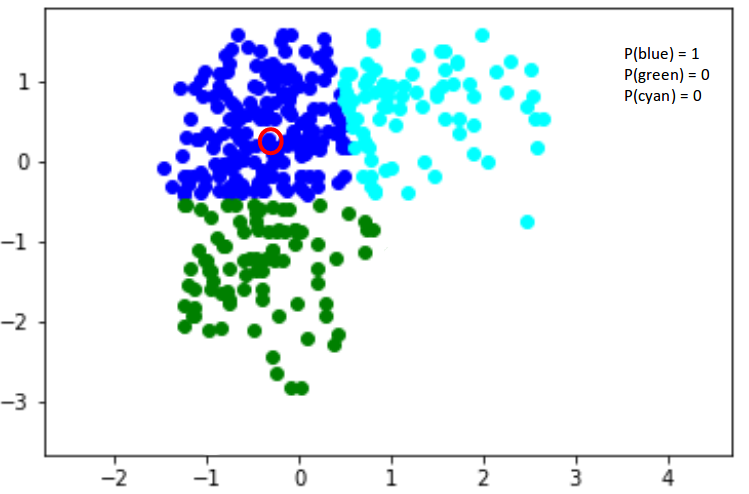
Here, we have three clusters that are denoted by three colors – Blue, Green, and Cyan. Let’s take the data point highlighted in red. The probability of this point being a part of the blue cluster is 1, while the probability of it being a part of the green or cyan clusters is 0.

These probabilities are computed using Bayes’ theorem, which relates the prior
and posterior probabilities of the cluster assignments given the data. An important decision in GMMs is choosing the appropriate number of components, which can be done using techniques like the Bayesian Information Criterion (BIC) or cross-validation.

Now, consider another point – somewhere in between the blue and cyan (highlighted in the below figure). The probability that this point is a part of cluster green is 0, right? The probability that this belongs to blue and cyan is 0.2 and 0.8 respectively. These coefficients represent the responsibilities or soft assignments of the data point to the different Gaussian components in the mixture.

 

Gaussian Mixture Models use the soft clustering technique for assigning data points to Gaussian distributions, leveraging Bayes’ theorem to compute the posterior probabilities. I’m sure you’re wondering what these distributions are so let me explain that in the next section.

The Gaussian Distribution

I’m sure you’re familiar with Gaussian Distributions (or the Normal Distribution). It has a bell-shaped curve, with the data points symmetrically distributed around the mean value.

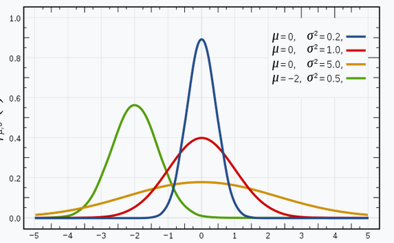
The below image has a few Gaussian distributions with a difference in mean (μ) and variance (σ 2 ). Remember that the higher the σ value more the spread:

 

 

 

 

Source: Wikipedia

In a one dimensional space, the probability density function of a Gaussian distribution is given by:

where μ is the mean and σ² is the variance.

But this would only be true for a single variable. In the case of two variables, instead of a 2D bell-shaped curve, we will have a 3D bell curve as shown below:

The probability density function would be given by:

where x is the input vector, μ is the 2D mean vector, and Σ is the 2×2 covariance matrix. The covariance would now define the shape of this curve. We can generalize the same for d-dimensions.

Thus, this multivariate Gaussian model would have x and μ as vectors of length d, and Σ would be a d x d covariance matrix.

Hence, for a dataset with d features, we would have a mixture of k Gaussian distributions (where k is equivalent to the number of clusters), each having a certain mean vector and variance matrix. But wait – how is the mean and variance value for each Gaussian assigned?

These values are determined using a technique called expectation maximization (EM). We need to understand this technique before we dive deeper into the working of Gaussian Mixture Models.

Characteristics of the Normal or Gaussian Distribution

Characteristics of the normal or Gaussian distribution:

• It’s bell-shaped with most values around the average.
• It has only one peak or mode.
• It stretches out forever in both directions.
• Its mean, median, and mode are the same.
• Its spread is measured by its standard deviation.
• The total area under its curve equals 1.