SUPPORT VECTOR MACHINES

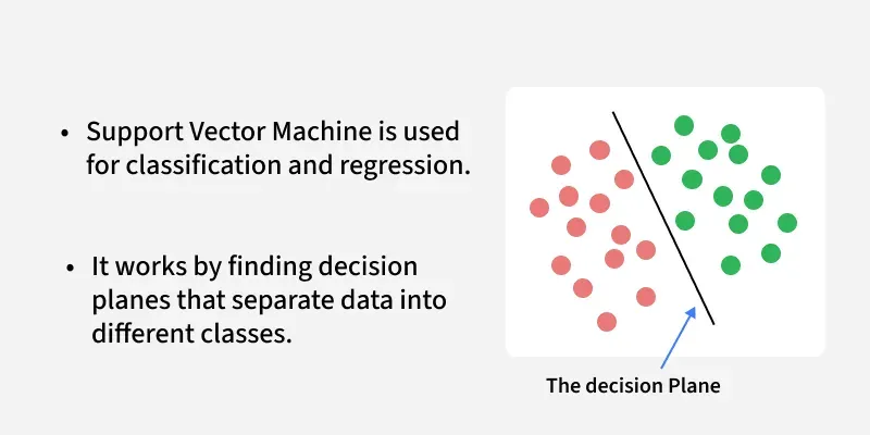
SVMs work by finding the optimal hyperplane that separates data points into different classes.

Key Terms

Hyperplane

A hyperplane is a decision boundary that separates data points into different classes in a high-dimensional space. In two-dimensional space, a hyperplane is simply a line that separates the data points into two classes. In three-dimensional space, a hyperplane is a plane that separates the data points into two classes. Similarly, in N-dimensional space, a hyperplane has (N-1)-dimensions.

It can be used to make predictions on new data points by evaluating which side of the hyperplane they fall on. Data points on one side of the hyperplane are classified as belonging to one class, while data points on the other side of the hyperplane are classified as belonging to another class.

Margin

A margin is the distance between the decision boundary (hyperplane) and the closest data points from each class. The goal of SVMs is to maximize this margin while minimizing classification errors. A larger margin indicates a greater degree of confidence in the classification, as it means that there is a larger gap between the decision boundary and the closest data points from each class. The margin is a measure of how well-separated the classes are in feature space. SVMs are designed to find the hyperplane that maximizes this margin, which is why they are sometimes referred to as maximum-margin classifiers.

Support Vectors

They are the data points that lie closest to the decision boundary (hyperplane) in a Support Vector Machine (SVM). These data points are important because they determine the position and orientation of the hyperplane, and thus have a significant impact on the classification accuracy of the SVM. In fact, SVMs are named after these support vectors because they “support” or define the decision boundary. The support vectors are used to calculate the margin, which is the distance between the hyperplane and the closest data points from each class. The goal of SVMs is to maximize this margin while minimizing classification errors.

Understanding SVM with an example dataset

A dataset with first 5 and last 5 rows, named “Iris” with columns sepal length, sepal width, petal length and petal width. — Iris Dataset from the Scikit-learn library in Python.

We have a famous dataset called ‘Iris’. There are four features (columns or independent variables) in this dataset but for simplicity purposes, we shall on look at two which are: ‘Petal length’ and ‘Petal Width’. These points are then plotted on a 2D plane.

Points from Iris dataset plotted in a 2D plane, along with 3 sets of linear classifiers (lines) [dotted, light and dark] trying to classify the data accurately. — Iris dataset separated by three lines (linear classifiers) represent by dark, light and dotted lines.

Lighter points represent the species ‘Iris Setosa’ and darker ones represent ‘Iris versicolor’.

We can simply classify this by plotting lines, using linear classifiers.

The dark and light lines accurately classify the test data set but may fail on new data due to the closeness of the boundary from the respective classes. Whereas, the dotted line classifier is entirely trash and misclassified many points.

What we want is the best classifier. A classifier which stays farthest from the overall class, that is where SVM comes in.

The same class of points separated by the resulting decision boundary of a SVM model. — Iris dataset separated by a hyperplane obtained by an SVM model.

We can think of SVM as fitting the widest possible path (represented by parallel dashed lines) between the classes.

This is termed “Large Margin Classification”.

Note. In theory, the hyperplane is exactly between the support vectors. But here it is slightly closer to the dark class. Why? This will be discussed later in the regularization part.

Understanding by an Analogy (You can skip if you understood :)

You can think of SVM as a construction company. The 2D plane is a map and the 2 classes are 2 cities. The data points are analogous to buildings. You are the government and your goal is to create the best highway to minimise traffic which passes through both the cities, but you are constrained by the area available to you.

We are considering the road to be “straight” for now. (We will explore non-linear models later in the article)

You give the contract to SVM construction company. What SVM does to minimise traffic is it wants to maximise the width of the road. It looks at the widest stretch of land between the 2 cities. The buildings at the end of the road are called “Support Vectors” since they are constraining or “Supporting” the model. The highway is angled such that there is equal space for the cities to expand along it.

This central line dividing the highway represents the Decision Boundary (Hyperplane) and the edges represent Hyperplanes for the respective Classes. The width of this highway is the Margin.

What Happens if the data is not linearly classifiable?

When a linear hyperplane is not possible, the input data is transformed into a higher-dimensional feature space, where it may be easier to find a linear decision boundary that separates the classes.

What do I mean by that 😕 ?

Let’s look at an example:

A set of points plotted in the 2-D plane divided into classes (red and yellow) arranged in concentric circular regions. Yellow points start from the origin and continue till a distance as points on the circumference of concentric circles. Then after a gap, the red points start which are plotted like yellow ones. There is a circle in between them acting as a hyperplane to separate the classes. — A dataset which is not linearly separable.

In the above figure, a 2-D hyperplane was not possible and hence transformation was required (remember I told you the case if the highway wasn’t straight).

What is transformation or addition of a new feature?

We have two features X and Y, and the data which not linearly classifiable. What we need to do is add another dimension in which if the data is plotted it becomes linearly separable.

Values of a point in the dimensions are nothing but column values of the point. To add another dimension we have to create another column (or feature).

Here we have two features X and Y, a third feature is needed which will be a function of the original features i.e. X and Y, which will be enough to classify the data linearly in three dimensions.

We take the third feature Z = f(x,y); f representing a function on X and Y. Here the Radial Basis Function(RBF) (measuring Euclidean distance) from the origin is enough.

Z = (X²+ Y²)^(1/2)

The 2D set of red and yellow points plotted in 3D, with distance from the origin as the third feature, now it is linearly classifiable as shown with a 2D plane (representing the hyperplane). — The points, plotted in 3-D with a hyperplane dividing them

Here the hyperplane was as simple as creating a plane parallel to the X-Y plane at a certain height.

Problems with this method

The main problem here is the heavy load of the calculations to be performed.

Here we took points centred on origin in a concentric manner. Suppose the points were not concentric but could be separated by the RBF. So we would need to take each point in the dataset as a reference each time and find the distance of all other points with respect to that point.

So we would need to calculate n*(n-1)/2 distances. (n-1 other points with respect to each n points, but once the distance of 1–2 is calculated the distance of 2–1 does need to be calculated)

Time Complexity

The time complexity of a square root is O(log(n)) and for power, addition is O(1). Thus to do n*(n-1)/2 total calculations we would need O(n²log(n)) time complexity.

But as our goal is to separate the classes and not find the distance, we can do away with the square root. (Z = X²+ Y²)

In that case, we would get a time complexity of O(n²).

But this was not even the problem, the problem starts now

Here we knew which function was to be used. But there could be many functions with just the degree limited to 2 (X, Y, XY, X² and Y²).

We can use these 5 as 3 dimensions in ⁵C₃ ways = 10 ways. Not to mention, the infinite possibility of their linear combinations (Z = 4X² + 7XY + 13Y², Z= 8XY +17X², and so on…).

And this was only for 2-degree polynomials. If we started using 3-degree polynomials then X³, Y³, X²Y, XY² will also come in the picture.

Not all of these are good enough to be our additional feature.

For example, I started with (X vs Y vs XY as the features):

A plot of the same dataset with X, Y and XY as the features. Figure looks like two birds have touched their beaks, with birds being the red class and their beaks yellow. This data in this form is not linearly classifiable. — X vs Y vs XY plot of the same data, this plot is not linearly classifiable [Doesn’t the figure look like two birds that have touched their beaks].

All the calculations and computations that went into this plot were in vain.

Now we have to use another function as the feature and try again.

Say, I use (X²+vs Y² vs XY as the features, yes I replaced X and Y):

A plot of the same dataset with X², Y² and XY as the features. The figure looks like a bird with its beak, with birds being the red class and its beak being yellow. This data in this form is linearly classifiable. — X² vs Y² vs XY plot of the same data, this plot is linearly classifiable [Doesn’t the figure look like a bird with its beak].

I saw that earlier data and noticed that it wasn't linearly separable since yellow was in between the red points.

Since the two yellow beaks met at the centre and one of them was going in the negative X and negative Y direction, I decided to square X and Y so that a new set of values begin from 0 forming only a single separation region between the beak and the bird’s face as compared to two earlier.

This plot is linearly separable, in this way, we can reuse the XY calculations and plot smartly to get the desired features to separate the data.

But even this has limitations, such as using only one or two feature datasets so we get a plot in 3-d and not more dimensions, also our brain's capacity to look for patterns to identify the next set of features and what if the first plot had no pattern so we had to again take a guess for a feature and start from scratch.

If we got the desired feature set in only two steps as we got above, even then this method is slower than the one we actually use.

What we use is called the Kernel Trick.

The Kernel Trick

A Kernel Trick instead of adding another dimension/feature, finds the similarity of the points.

Instead of finding f(x,y) directly, it computes the similarity of the image of these points. In other words, instead of finding f(x1,y1) and f(x2,y2) we take the points (x1,y1) and (x2,y2) and compute how similar would their outputs be using a function f(x,y); where f can be any function on x,y.

Thus we don’t need to find a suitable set of features here. We find similarity in such a way that it is valid for all sets of features.

To calculate the similarity we use the Gaussian function.

f(x) = ae^(-(x-b)²/2c²)
a : represents the height of the peak of the curve
b : represents the position of the centre of the peak
c : is the standard deviation of the data

For RBF Kernel we use:

K(X,X’) = e^-γ(|X-X’|²) = (1/ e^|X-X’|²) γ
γ : is a hyperparameter which represents the linearlity of the model (γ ∝ 1/c²)
X,X’ :represents the position vectors of the two points

A small γ (tending to 0) means a more linear model and a large γ means a more non-linear model.

Here we have 2 models (left with γ = 1 and right with γ = 0.01, much more linear in nature).

Two SVM models with different γ, on the left model, is highly curved and matches the data whereas on the right model is more linear in nature. — Two Models with Different Gamma Values.

So why not let gamma be a very high value? What is the use of a low γ?

Large values of gamma may lead to overfitting as well and thus we need to find appropriate gamma values.

Figure with 3 models, from left γ = 0.1, γ = 10, γ = 100. (The left one is accurately fitted, the middle is overfitted and the right one is extremely overfitted)

Three SVM models with different γ, the left model, is accurately curved and has appropriate γ value, the middle and the right model has a even higher value of γ thus they have overfitted the data. — Three Models with Different Gamma Values.

Time Complexity

Since we need to find the similarity of each point with respect to all other points we need a total of n*(n-1)/2 calculations.

Exponent has a time complexity of O(1) and thus we get a total time complexity of O(n²).

We do not need to plot points, check feature sets, take combinations, etc. This makes this method way more efficient.

What we do have here is the usage of different Kernels for this.

We have Kernels such as:

Polynomial Kernel
Gaussian Kernel
Gaussian RBF Kernel
Laplace RBF Kernel
Hyperbolic Tangent Kernel
Sigmoid Kernel
Bessel function of first kind Kernel
ANOVA radial basis Kernel
Linear Splines Kernel

Whichever one we use, we get results in lesser computations than the original method.

To further optimise our calculations we use the “Gram Matrix”.

The Gram Matrix is a matrix which can be easily stored and manipulated in the memory and is highly efficient to use.

Regularization and Soft Margin SVM

Finally, Onto a new topic 😮‍💨(phew).

If we strictly impose that all points must be off the street on the correct side then this is called Hard Margin Classification (remember the first SVM model figure that I showed).

There are two issues with this method. First, it would only work with linearly separable data and not for non-linearly separable data (which may be linearly classifiable for the most part).

Second, is its sensitivity to outliers. In the figure below the Red Point is introduced as an outlier in the left class and it significantly changes the decision boundary, this may result in misclassifications of non-outlier data of the second class while testing the model.

The first “Iris” dataset with an outlier introduced in the left class which is very close to the second class and ends up completely changing the decision boundary and hyper planes — The “Iris” dataset with an outlier completely changes the decision hyperplane.

Although this model has not misclassified any of the points it is not a very good model and will give higher errors during testing.

To avoid this, we use Soft Margin Classification.

A soft margin is a type of margin that allows for some misclassification errors in the training data.

“Iris” dataset with the outlier but with Soft Margin Classification, and misclassifying the outlier on purpose — “Iris” dataset with the outlier but with Soft Margin Classification.

Here, a soft margin allows for some misclassification errors by allowing some data points to be on the wrong side of the decision boundary.

Even though there is a misclassification in the training data set and worse performance with respect to the previous model, the general performance would be much better during testing, as a result of how far it is from both classes.

But we can solve the problem of outliers by removing them using data preprocessing and data cleaning right? Then why Soft Margins?

They are used mainly when the data is not linearly separable, meaning that it is not possible to find a hyperplane that perfectly separates the classes without any errors and to avoid outliers (Hard Margin Classification is not possible). Example :

“Iris” Datset (Right class is Iris Virginica, Left Class is Iris Versicolor), not linearly separable. (Value of C = 100) — “Iris” dataset (Right Class is Iris Virginica, Left Class is Iris Versicolor), is non-linearly separable but when Soft Margin Classification is used, we get a model with minimum misclassification. (0 minor misclassifications with respect to hyperplanes of respective classes) [5 major misclassifications, wrong side of decision boundary] (Value of C = 100).

How are Soft Margins working?

Soft margins are implemented by introducing a slack variable for each data point, which allows the SVM to tolerate some degree of misclassification error. The amount of tolerance is controlled by a parameter called the regularization hyperparameter C, which determines how much weight should be given to minimizing classification errors versus maximizing the margin.

It controls how much tolerance is allowed for misclassification errors, with larger values of C leading to a harder margin (less tolerance for errors) and smaller values of C leading to a softer margin (more tolerance for errors).

Basically through our analogy, instead of creating a very small road (for the outlier case) when it was not possible to create a large road through the middle of the two cities we create a larger road by moving out some people.

It may be bad for the people moving out (the outlier getting misclassified) but overall the highway (our model) would be way larger (more accurate) and better.

In the case above where no road could be created, we ask some people to move out and create a narrow road. A wider road though better for transport would cause problems for a large number of people (many points getting misclassified).

The regularization hyperparameter ‘C’ controls how many people can be moved out (how many points can be misclassified or tolerance) for the construction of the project.

A high value of C means the model is harder in nature (less tolerant to misclassifications). Whereas a low value of C means that the model is softer in nature (more tolerant to misclassifications).

Last Model but with the value of C = 1, a wider margin (more misclassifications) — Same Model with the value of C = 1 (12 minor misclassifications with respect to hyperplane of the classes) [4 major misclassifications, wrong side of decision boundary].

A lower C value for the previous model (1 with respect to 100) tolerates more misclassifications, allowing more people to move out and thus building a wider street).

Note. Lower value of C does not necessarily mean more major misclassifications always, sometimes it may mean way more minor classifications.

In this case and for most general cases, low values of C tend to give trash models misclassifying multiple points and reducing accuracy.

Note. A low C is not simply just widening the original path until the required tolerance level is met. It means creating a new widest path by misclassifying the maximum number of points such that it is below the tolerance threshold.

C controls the Bias/Variance trade-off. A low bias means that the model has low or no assumptions about the data. A high variance means that the model will change depending on what we take as training data.

For Hard Margin Classification, the model changes significantly on changing data (if new points were introduced between the hyperplanes) so it has high variance, but it has no assumption about the data there is low bias.

Soft Margin Classification models have negligible changes (due to tolerance to misclassify data) thus they have a low variance. But it assumes we can misclassify some information and assumed that the particular model with a wider margin would lead to better results and thus have a high bias.

Why use low value of C then? Why an appropriate value needs to be chosen

This is a phenomenon similar to overfitting and underfitting which happens with very high values of C and very low values of C.

Very low values will give very poor results as seen (similar to the case of underfitting).

Modified “Iris” dataset used in the first model to show overfitting, with C = 1000 — Modified dataset to show the phenomenon.

Model with C = 1000, is unsuitable as it is too close to the left class at the bottom and too close to the right class at the top, with chances of misclassifying data (here there is only 1 major misclassification and 1 minor misclassification hence, during training the model is good, but the model is not good for general decision making and may perform poorly during testing).

Thus models with a very high value of C may also give poor results on testing (similar to the case of overfitting).

Modified “Iris” dataset used, but here with C = 1.

Model with C = 1, suitable and better-generalised model. (Though there are 3 major misclassifications and about 12 minor misclassifications and thus a worse performance on training data but the model keeps in mind the bulk of the data and creates decision boundaries according to that, hence it has better performance during testing owing to its distance from both the classes).

Note: Minor misclassification is a term which I use to describe data not correctly classified by the class’ hyperplane. They do not lead to worse performance directly but give an indicator that the model may be worse. Hence in the above case despite 15 misclassifications performance is not 7.5 times worse, but only 3 times worse on training data due to 3 times more major misclassifications.

Remember I said initially about how in theory the decision boundary shall be in between the support vectors, but it was slightly closer to the darker class. That, was due to regularization. It created a model with 2 minor misclassifications such that the overall model is a more accurate one.

And thus the model should have been represented like this:

Corrected version of the first model, with 2 minor misclassifications (Decision Boundary is now equidistant from the support vectors).

Regression using SVM

SVMs, although generally used for classification can be used for both regression and classification. Support Vector Regression (SVR) is a machine learning algorithm used for regression analysis. It is different from traditional linear regression methods as it finds a hyperplane that best fits the data points in a continuous space, instead of fitting a line to the data points.

SVR in contrast to SVM tries to maximise the number of points in the street (margin), the width is controlled by a hyperparameter ε (epsilon).

An Image displaying suport vector regression where the margin encompasses the points and the decision hyperplane is used to predict the value and how it can do regression non linearly using kernel trick. — Support Vector Regression (SVR) the decision hyperplane is used to predict the value.

An analogy of this could be passing a flyover or a bridge over buildings or houses where we want to give shade to the most number of houses keeping the bridge thinnest.

SVR wants to include the whole data into its reach while trying to minimise the margin, basically trying to encompass the points. Whereas linear regression wants to pass a line such that the sum of distances of the points from the line is minimum.

The advantages of SVR over normal regression are:

Non-linearity: SVR can capture non-linear relationships between input features and the target variable. It achieves this by using the kernel trick. In contrast, Linear Regression assumes a linear relationship between the input features and the target variable and Non-Linear Regression would require a lot of computation.
Robustness to outliers: SVR is more robust to outliers compared to Linear Regression. SVR aims to minimize the errors within a certain margin around the predicted values, known as the epsilon-insensitive zone. This characteristic makes SVR less influenced by outliers that fall outside the margin, leading to more stable predictions.
Sparsity of support vectors: SVR typically relies on a subset of training instances called support vectors to construct the regression model. These support vectors have the most significant impact on the model and represent the critical data points for determining the decision boundary. This sparsity property allows SVR to be more memory-efficient and computationally faster than Linear Regression, especially for large datasets. Also, an advantage is that after the addition of new training points the model does not change if they lie in the margin.
Control over model complexity: SVR provides control over model complexity through hyperparameters such as the regularization parameter C and the kernel parameters. By adjusting these parameters, you can control the trade-off between model complexity and generalization ability this level of flexibility is not offered by linear regression.

Applications and Uses of SVM

Support Vector Machines (SVMs) have been successfully applied to various real-world problems across different domains. Here are some notable applications of SVMs:

Image Classification: SVMs have been widely used for image object recognition, handwritten digit recognition and optical character recognition (OCR). They have been employed in systems like filtering image-based spam and face detection systems used for security, surveillance, and biometric identification.
Text Classification: SVMs are effective for text categorization tasks, such as sentiment analysis, spam detection, and topic classification.
Bioinformatics: SVMs have been applied in bioinformatics for tasks such as protein structure prediction, gene expression analysis, and DNA classification.
Financial Forecasting: SVMs have been used in financial applications for tasks such as stock market prediction, credit scoring, and fraud detection.
Medical Diagnosis: SVMs have been utilized in medical diagnosis and decision-making systems. They can assist in diagnosing diseases, predicting patient outcomes, or identifying abnormal patterns in medical images.

SVMs have also been applied in other domains such as geosciences, marketing, computer vision, and more, showcasing their versatility and effectiveness in various problem domains.

Support Vector Machine (SVM) is a supervised machine learning algorithm used for classification and regression tasks. It tries to find the best boundary known as hyperplane that separates different classes in the data. It is useful when you want to do binary classification like spam vs. not spam or cat vs. dog.

The main goal of SVM is to maximize the margin between the two classes. The larger the margin the better the model performs on new and unseen data.

Key Concepts of Support Vector Machine

Hyperplane: A decision boundary separating different classes in feature space and is represented by the equation wx + b = 0 in linear classification.
Support Vectors: The closest data points to the hyperplane, crucial for determining the hyperplane and margin in SVM.
Margin: The distance between the hyperplane and the support vectors. SVM aims to maximize this margin for better classification performance.
Kernel: A function that maps data to a higher-dimensional space enabling SVM to handle non-linearly separable data.
Hard Margin: A maximum-margin hyperplane that perfectly separates the data without misclassifications.
Soft Margin: Allows some misclassifications by introducing slack variables, balancing margin maximization and misclassification penalties when data is not perfectly separable.
C: A regularization term balancing margin maximization and misclassification penalties. A higher C value forces stricter penalty for misclassifications.
Hinge Loss: A loss function penalizing misclassified points or margin violations and is combined with regularization in SVM.
Dual Problem: Involves solving for Lagrange multipliers associated with support vectors, facilitating the kernel trick and efficient computation.

How does Support Vector Machine Algorithm Work?

The key idea behind the SVM algorithm is to find the hyperplane that best separates two classes by maximizing the margin between them. This margin is the distance from the hyperplane to the nearest data points (support vectors) on each side.

SVM — Multiple hyperplanes separate the data from two classes

The best hyperplane also known as the "hard margin" is the one that maximizes the distance between the hyperplane and the nearest data points from both classes. This ensures a clear separation between the classes. So from the above figure, we choose L2 as hard margin. Let's consider a scenario like shown below:

Selecting hyperplane for data with outlier

Here, we have one blue ball in the boundary of the red ball.

How does SVM classify the data?

The blue ball in the boundary of red ones is an outlier of blue balls. The SVM algorithm has the characteristics to ignore the outlier and finds the best hyperplane that maximizes the margin. SVM is robust to outliers.

Hyperplane which is the most optimized one

A soft margin allows for some misclassifications or violations of the margin to improve generalization. The SVM optimizes the following equation to balance margin maximization and penalty minimization:

$Objective Function = (\frac{1}{margin}) + λ \sum penalty$

The penalty used for violations is often hinge loss which has the following behavior:

If a data point is correctly classified and within the margin there is no penalty (loss = 0).
If a point is incorrectly classified or violates the margin the hinge loss increases proportionally to the distance of the violation.

Till now we were talking about linearly separable data that seprates group of blue balls and red balls by a straight line/linear line.

What if data is not linearly separable?

When data is not linearly separable i.e it can't be divided by a straight line, SVM uses a technique called kernels to map the data into a higher-dimensional space where it becomes separable. This transformation helps SVM find a decision boundary even for non-linear data.

A kernel is a function that maps data points into a higher-dimensional space without explicitly computing the coordinates in that space. This allows SVM to work efficiently with non-linear data by implicitly performing the mapping. For example consider data points that are not linearly separable. By applying a kernel function SVM transforms the data points into a higher-dimensional space where they become linearly separable.

Linear Kernel: For linear separability.
Polynomial Kernel: Maps data into a polynomial space.
Radial Basis Function (RBF) Kernel: Transforms data into a space based on distances between data points.

Mapping 1D data to 2D to become able to separate the two classes

In this case the new variable y is created as a function of distance from the origin.

Mathematical Computation of SVM

Consider a binary classification problem with two classes, labeled as +1 and -1. We have a training dataset consisting of input feature vectors X and their corresponding class labels Y. The equation for the linear hyperplane can be written as:

$w^{T} x + b = 0$

Where:

$w$ is the normal vector to the hyperplane (the direction perpendicular to it).
$b$ is the offset or bias term representing the distance of the hyperplane from the origin along the normal vector $w$ .

Distance from a Data Point to the Hyperplane

The distance between a data point $x_{i}$ and the decision boundary can be calculated as:

$d_{i} = \frac{w^{T} x_{i} + b}{∣ ∣ w ∣ ∣}$

where ||w|| represents the Euclidean norm of the weight vector w.

Linear SVM Classifier

Distance from a Data Point to the Hyperplane:

$\hat{y} = {\begin{array}{cl} 1 & : w^{T} x + b \geq 0 \\ - 1 & : w^{T} x + b < 0 \end{array}$

Where $\hat{y}$ is the predicted label of a data point.

Optimization Problem for SVM

For a linearly separable dataset the goal is to find the hyperplane that maximizes the margin between the two classes while ensuring that all data points are correctly classified. This leads to the following optimization problem:

$\underset{w, b}{minimize} \frac{1}{2} {∥ w ∥}^{2}$

Subject to the constraint:

$y_{i} (w^{T} x_{i} + b) \geq 1 f o r i = 1, 2, 3, \dots, m$

Where:

$y_{i}$ is the class label (+1 or -1) for each training instance.
$x_{i}$ is the feature vector for the $i$ -th training instance.
$m$ is the total number of training instances.

The condition $y_{i} (w^{T} x_{i} + b) \geq 1$ ensures that each data point is correctly classified and lies outside the margin.

Soft Margin in Linear SVM Classifier

In the presence of outliers or non-separable data the SVM allows some misclassification by introducing slack variables $ζ_{i}$ . The optimization problem is modified as:

$\underset{w, b}{minimize} \frac{1}{2} ∥ w ∥^{2} + C \sum_{i = 1}^{m} ζ_{i}$

Subject to the constraints:

$y_{i} (w^{T} x_{i} + b) \geq 1 - ζ_{i} and ζ_{i} \geq 0 for i = 1, 2, \dots, m$

Where:

$C$ is a regularization parameter that controls the trade-off between margin maximization and penalty for misclassifications.
$ζ_{i}$ are slack variables that represent the degree of violation of the margin by each data point.

Dual Problem for SVM

The dual problem involves maximizing the Lagrange multipliers associated with the support vectors. This transformation allows solving the SVM optimization using kernel functions for non-linear classification.

The dual objective function is given by:

$\max_{α} \frac{1}{2} \sum_{i = 1}^{m} \sum_{j = 1}^{m} α_{i} α_{j} t_{i} t_{j} K (x_{i}, x_{j}) - \sum_{i = 1}^{m} α_{i}$

Where:

$α_{i}$ are the Lagrange multipliers associated with the $i^{t h}$ training sample.
$t_{i}$ is the class label for the $i^{t h}$ -th training sample.
$K (x_{i}, x_{j})$ is the kernel function that computes the similarity between data points $x_{i}$ and $x_{j}$ . The kernel allows SVM to handle non-linear classification problems by mapping data into a higher-dimensional space.

The dual formulation optimizes the Lagrange multipliers $α_{i}$ and the support vectors are those training samples where $α_{i} > 0$ .

SVM Decision Boundary

Once the dual problem is solved, the decision boundary is given by:

$w = \sum_{i = 1}^{m} α_{i} t_{i} K (x_{i}, x) + b$

Where $w$ is the weight vector, $x$ is the test data point and $b$ is the bias term. Finally the bias term $b$ is determined by the support vectors which satisfy:

$t_{i} (w^{T} x_{i} - b) = 1 \Rightarrow b = w^{T} x_{i} - t_{i}$

Where $x_{i}$ is any support vector.

This completes the mathematical framework of the Support Vector Machine algorithm which allows for both linear and non-linear classification using the dual problem and kernel trick.

Types of Support Vector Machine

Based on the nature of the decision boundary, Support Vector Machines (SVM) can be divided into two main parts:

Linear SVM: Linear SVMs use a linear decision boundary to separate the data points of different classes. When the data can be precisely linearly separated, linear SVMs are very suitable. This means that a single straight line (in 2D) or a hyperplane (in higher dimensions) can entirely divide the data points into their respective classes. A hyperplane that maximizes the margin between the classes is the decision boundary.

Non-Linear SVM:Non-Linear SVM can be used to classify data when it cannot be separated into two classes by a straight line (in the case of 2D). By using kernel functions, nonlinear SVMs can handle nonlinearly separable data. The original input data is transformed by these kernel functions into a higher-dimensional feature space where the data points can be linearly separated. A linear SVM is used to locate a nonlinear decision boundary in this modified space.

Implementing SVM Algorithm Using Scikit-Learn

We will predict whether cancer is Benign or Malignant using historical data about patients diagnosed with cancer. This data includes independent attributes such as tumor size, texture, and others. To perform this classification, we will use an SVM (Support Vector Machine) classifier to differentiate between benign and malignant cases effectively.

load_breast_cancer(): Loads the breast cancer dataset (features and target labels).
SVC(kernel="linear", C=1): Creates a Support Vector Classifier with a linear kernel and regularization parameter C=1.
svm.fit(X, y): Trains the SVM model on the feature matrix X and target labels y.
DecisionBoundaryDisplay.from_estimator(): Visualizes the decision boundary of the trained model with a specified color map.
plt.scatter(): Creates a scatter plot of the data points, colored by their labels.
plt.show(): Displays the plot to the screen.

from sklearn.datasets import load_breast_cancer
import matplotlib.pyplot as plt
from sklearn.inspection import DecisionBoundaryDisplay
from sklearn.svm import SVC

cancer = load_breast_cancer()
X = cancer.data[:, :2]
y = cancer.target

svm = SVC(kernel="linear", C=1)
svm.fit(X, y)

DecisionBoundaryDisplay.from_estimator(
        svm,
        X,
        response_method="predict",
        alpha=0.8,
        cmap="Pastel1",
        xlabel=cancer.feature_names[0],
        ylabel=cancer.feature_names[1],
    )

plt.scatter(X[:, 0], X[:, 1], 
            c=y, 
            s=20, edgecolors="k")
plt.show()

Output:

Advantages of Support Vector Machine (SVM)

High-Dimensional Performance: SVM excels in high-dimensional spaces, making it suitable for image classification and gene expression analysis.
Nonlinear Capability: Utilizing kernel functions like RBF and polynomial SVM effectively handles nonlinear relationships.
Outlier Resilience: The soft margin feature allows SVM to ignore outliers, enhancing robustness in spam detection and anomaly detection.
Binary and Multiclass Support: SVM is effective for both binary classification and multiclass classification suitable for applications in text classification.
Memory Efficiency: It focuses on support vectors making it memory efficient compared to other algorithms.

Disadvantages of Support Vector Machine (SVM)

Slow Training: SVM can be slow for large datasets, affecting performance in SVM in data mining tasks.
Parameter Tuning Difficulty: Selecting the right kernel and adjusting parameters like C requires careful tuning, impacting SVM algorithms.
Noise Sensitivity: SVM struggles with noisy datasets and overlapping classes, limiting effectiveness in real-world scenarios.
Limited Interpretability: The complexity of the hyperplane in higher dimensions makes SVM less interpretable than other models.
Feature Scaling Sensitivity: Proper feature scaling is essential, otherwise SVM models may perform poorly.

CrazyLearners🙂

Search This Blog